Digging into BVB Dortmund Football Club's Tweets with R
December 12, 2020 - 18 minutes
tidyverse r rstats gt rtweet ggmapPurpose
The goal of this post is to source and analyze Twitter posts and followers for a given Twitter account (“handle”) using R. We will identify tweets with the most likes and retweets, as well as posting trends over time. We will also map the geographic distribution of Twitter followers by leveraging Google Maps API attributes.
The example Twitter handle will be the English language account of BVB Dortmund (“BVB”), a football team in Germany’s top professional league, the Bundesliga. We are using BVB’s English Twitter account instead of the club’s primary German language Twitter account because this blog post is written in English.
1. Setup
First, we need to obtain and authorize a free Twitter Developer account (instructions here).
Second step is to install and load the R rtweet package by Michael Kearney.
We will extract Twitter data multiple times so I have created two variables to avoid duplication and inconsistencies. The “twitter_user” variable stores the Twitter handle. The “sample” variable specifies the number of extracted records as some Twitter accounts have large volumes of followers and tweets.
   library (rtweet)
   library (tidyverse)

   twitter_user <- "@blackyellow"
2. Analyze tweets
Source tweets
Now we will extract our first set of Twitter data.
The get_timeline function contains 90 fields for each tweet. The BVB account posts frequently so we will limit to the last 500 tweets.
tweets_raw <- get_timeline (twitter_user, n = 500)Transform Tweets
Many fields are not needed for this exercise so we can cull the dataset. I have also renamed several fields for brevity and more standard Twitter notation (i.e. likes instead of favorites).
We are focusing on original tweets so have filtered out retweets.
I have extracted year from the creation date to enable summarizing tweet volume by year. Also, I have truncated the Tweet text field from 280 to 60 characters so more cleanly fits in a formatted table.
   library (lubridate)

   tweets <- tweets_raw %>%
      filter (is_retweet == FALSE) %>%
      rename (
         likes = favorite_count,
         retweets = retweet_count,
         created = created_at
         ) %>%
      mutate (
         text = str_sub(text,1,60),
         created = as.Date(created),
         year = year(created)
         ) %>%
      rename(date = created) %>%
      select (text, date, year, likes, retweets)
Visualize most liked tweets
We will sort by most liked tweets over time and rank via the dplyr row_to_column formula.
The GT package by Richard Iannone formats tables in a easy-to-read manner. The core gt::gt function adds lines between rows. Many other table formatting enhancements are available but out of scope for this blog.
The tweet with the most likes was BVB’s tribute to football legend Diego Maradona, who recently passed away.
   library (gt)

   tweets %>%
      arrange (-likes, -retweets) %>%
      head (10) %>%
      rowid_to_column("rank") %>%
      select (-year) %>%
      relocate (rank) %>%
gt () | rank | text | date | likes | retweets |
|---|---|---|---|---|
| 1 | Rest In Peace, Diego Armando Maradona 🙏 https://t.co/JB0DiVE | 2020-11-25 | 39014 | 2541 |
| 2 | Your 2020 Golden Boy Award Winner: ⭐️ ERRRRRLIIINNNGG HAAAA | 2020-11-21 | 25891 | 1462 |
| 3 | “Only two?” 😂 https://t.co/OHcaIkNGnt | 2020-11-24 | 23054 | 1004 |
| 4 | He is not real. | 2020-11-21 | 21004 | 1010 |
| 5 | Just another day in the office 🎮 https://t.co/yE1IpiC6gc | 2020-11-26 | 19328 | 359 |
| 6 | He's the Golden Boy for a reason | 2020-11-21 | 16180 | 788 |
| 7 | The Goalden Boy 🥅⚽️ https://t.co/XgIiDyKcC2 | 2020-11-22 | 13386 | 354 |
| 8 | Hakuna Matata - Marco Reus 🤙 https://t.co/PlTGdBLrhg | 2020-11-28 | 12865 | 1520 |
| 9 | Are you excited for the international break to end? Yes | 2020-11-18 | 12741 | 494 |
| 10 | Sweet Sixteen, Youssoufa Moukoko 🥳🎂 https://t.co/UaGEFhV0hC | 2020-11-20 | 11921 | 385 |
Visualize most retweeted tweets
Next we will re-sort and re-rank by retweets, again using the GT package to cleanly format.
A tweet celebrating player striker Giovanni Reyna signing a contract extension produced the most retweets. The tribute to Argentine football legend Diego Maradona (most liked tweet) was #2 when ranking by retweets.
   tweets %>%
      arrange (-retweets, -likes) %>%
      head (10) %>%
      rowid_to_column("rank") %>%
      select (rank, text, date, retweets, likes) %>%
gt ()| rank | text | date | retweets | likes |
|---|---|---|---|---|
| 1 | 🚨 #REYNA2025 GIVEAWAY 🚨 To celebrate Gio’s contract extensi | 2020-11-21 | 4926 | 3327 |
| 2 | Rest In Peace, Diego Armando Maradona 🙏 https://t.co/JB0DiVE | 2020-11-25 | 2541 | 39014 |
| 3 | Hakuna Matata - Marco Reus 🤙 https://t.co/PlTGdBLrhg | 2020-11-28 | 1520 | 12865 |
| 4 | Your 2020 Golden Boy Award Winner: ⭐️ ERRRRRLIIINNNGG HAAAA | 2020-11-21 | 1462 | 25891 |
| 5 | He is not real. | 2020-11-21 | 1010 | 21004 |
| 6 | “Only two?” 😂 https://t.co/OHcaIkNGnt | 2020-11-24 | 1004 | 23054 |
| 7 | 63 | HAATTRICK!!! THIS MAN IS NOT HUMAN!!! #BSCBVB 1-3 htt | 2020-11-21 | 844 | 10091 |
| 8 | He's the Golden Boy for a reason | 2020-11-21 | 788 | 16180 |
| 9 | Just had to make sure 🤖 https://t.co/xScWp4Taw1 | 2020-11-21 | 749 | 7233 |
| 10 | The last time we faced Frankfurt...💛🏟 https://t.co/hlg7Z18Dl | 2020-12-04 | 597 | 11384 |
Visualize number of tweets trends
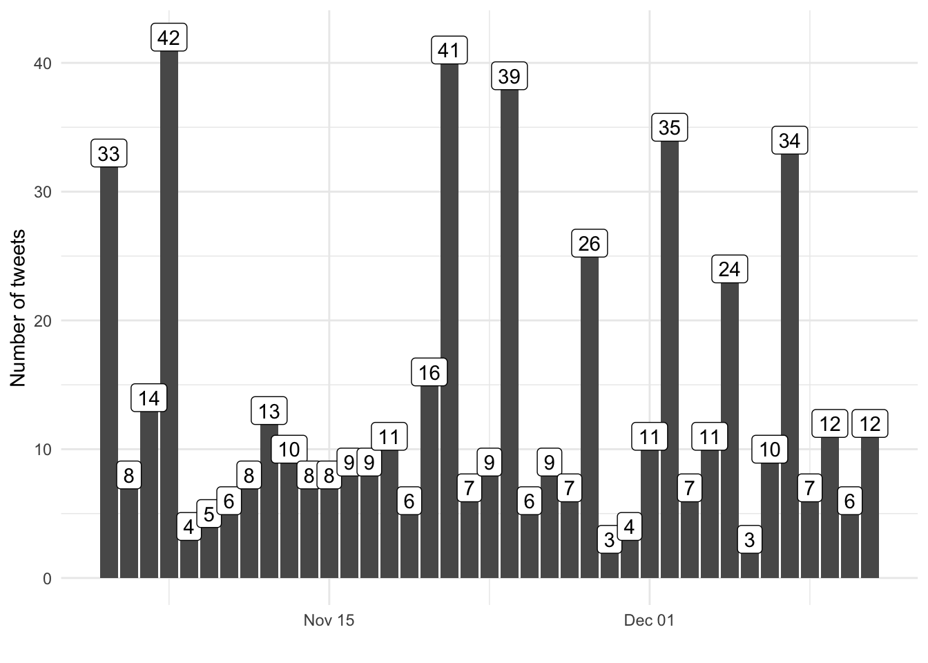
Another area of interest is how tweet activity has evolved over time. Using dplyr we can easily summarize by number of tweets by day.
The volume of tweets was smallest during the international break in early to mid November. BVB does not play games during international breaks because the players are away representing their respective national football teams.
   tweets %>%
      group_by (date) %>%
      count () %>%
      ggplot (aes (x = date, y = n)) +
         geom_col () +
         geom_label (aes(label = n)) +
         theme_minimal() +
         labs (x="", y = "Number of tweets")
3. Analyze Twitter followers
Source followers
Learning about followers for a Twitter handle is also frequently useful.
Two rtweet package functions are helpful here. First, get_followers returns a vector of Twitter user_ids of followers. The lookup_users function then extracts user attributes such as screen name, physical location (if supplied in profile) and number of followers.
The BVB account enjoys 583,000 followers so we will limit to 500 users for this blog entry. This is not a representative sample and is provided for illustrating R’s visualization capabilities.
We will also add a row ID ranking each follower by largest number of followers via dplyr’s rowid_to_column function.
   library(skimr)

  followers <- twitter_user %>%
      get_followers() %>%
      head (500) %>%
      pull (user_id) %>%
      lookup_users () %>%
      select (screen_name, name, location, followers_count) %>%
      arrange (-followers_count) %>%
      rowid_to_column("rank")

skim (followers)| Name | followers |
| Number of rows | 500 |
| Number of columns | 5 |
| _______________________ | |
| Column type frequency: | |
| character | 3 |
| numeric | 2 |
| ________________________ | |
| Group variables | None |
Variable type: character
| skim_variable | n_missing | complete_rate | min | max | empty | n_unique | whitespace |
|---|---|---|---|---|---|---|---|
| screen_name | 0 | 1 | 5 | 15 | 0 | 500 | 0 |
| name | 0 | 1 | 0 | 46 | 1 | 500 | 0 |
| location | 0 | 1 | 0 | 30 | 339 | 151 | 0 |
Variable type: numeric
| skim_variable | n_missing | complete_rate | mean | sd | p0 | p25 | p50 | p75 | p100 | hist |
|---|---|---|---|---|---|---|---|---|---|---|
| rank | 0 | 1 | 250.50 | 144.48 | 1 | 125.75 | 250.5 | 375.25 | 500 | ▇▇▇▇▇ |
| followers_count | 0 | 1 | 212.32 | 1636.84 | 0 | 1.00 | 8.0 | 46.25 | 30252 | ▇▁▁▁▁ |
Top followers
We will first list the 10 largest followers by respective number of followers.
The follower from the sample with the most followers is winnie.
   followers %>%
      head (10) %>%
      select (rank, name, location, followers_count) %>%
      gt () %>%
fmt_number (columns = vars(followers_count), use_seps = T, decimals = 0)| rank | name | location | followers_count |
|---|---|---|---|
| 1 | Spence Checketts | Salt Lake City, Utah | 30,252 |
| 2 | شوقي | 16,916 | |
| 3 | James Fielden | London | 9,751 |
| 4 | 11.01🥂🎈 | Pretoria, South Africa | 3,386 |
| 5 | feyyaz | Sanliurfa, Turkey | 2,802 |
| 6 | Biyan Rizaldy | Indonesia | 2,800 |
| 7 | Ashwin Appiah | Seattle, WA | 2,592 |
| 8 | TheGreekMamba 🇬🇷🇨🇦 | Toronto, Ontario | 2,358 |
| 9 | Likes&Retweets | Nigeria | 2,009 |
| 10 | Dj Irakoze | Kampala, Uganda | 1,951 |
Obtain follower geographic attributes
Another interesting item to research on followers is geographic distribution.
The provided location in Twitter profile is a good starting point. However, locations are neither standardized by level of detail (city, country) nor spelling. Standardization is necessary to group in table or map.
We will standardize at the highest level of detail, which is country, via the Google Maps API and accessed via the ggmaps package. If this is the first time you have accessed the Google Maps API, you will need to complete a one-time step of obtaining a free Google maps API key (instructions here).
   library (ggmap)

   register_google(key = Sys.getenv("GOOGLE_MAPS_API"))

   followers_geo <- followers %>%
      mutate_geocode (location, output = "more") %>%
      mutate (
         country = word (address, -1, -1, sep = ","),
         country = str_to_upper (country),
         country = str_trim(country),
         country = ifelse(is.na(country), "NOT LISTED", country)
         ) %>%
      select (rank:followers_count, country, address, lon, lat)

   followers_geo
## # A tibble: 500 x 9
## rank screen_name name location followers_count country address lon
## <int> <chr> <chr> <chr> <int> <chr> <chr> <dbl>
## 1 1 spencechec… Spen… "Salt L… 30252 USA salt l… -112.
## 2 2 shawkiii14 شوقي "" 16916 NOT LI… <NA> NA
## 3 3 James_Fiel… Jame… "London" 9751 UK london… -0.128
## 4 4 MalomaPale… 11.0… "Pretor… 3386 SOUTH … pretor… 28.2
## 5 5 feyyyaz feyy… "Sanliu… 2802 TURKEY şanlıu… 38.8
## 6 6 biyanrizal… Biya… "Indone… 2800 INDONE… indone… 114.
## 7 7 ashwinappi… Ashw… "Seattl… 2592 USA seattl… -122.
## 8 8 TheGreekMa… TheG… "Toront… 2358 CANADA toront… -79.4
## 9 9 folamisegun Like… "Nigeri… 2009 NIGERIA nigeria 8.68
## 10 10 DeejayIrak… Dj I… "Kampal… 1951 UGANDA kampal… 32.6
## # … with 490 more rows, and 1 more variable: lat <dbl>Visualize followers by country
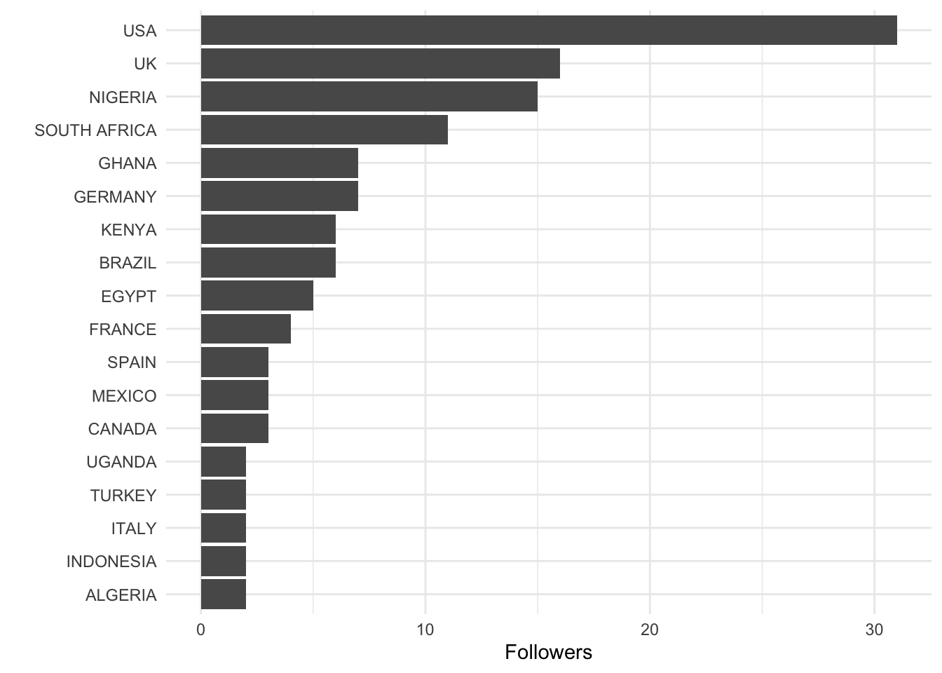
We will first identify the top follower countries and summarize in a GT table.
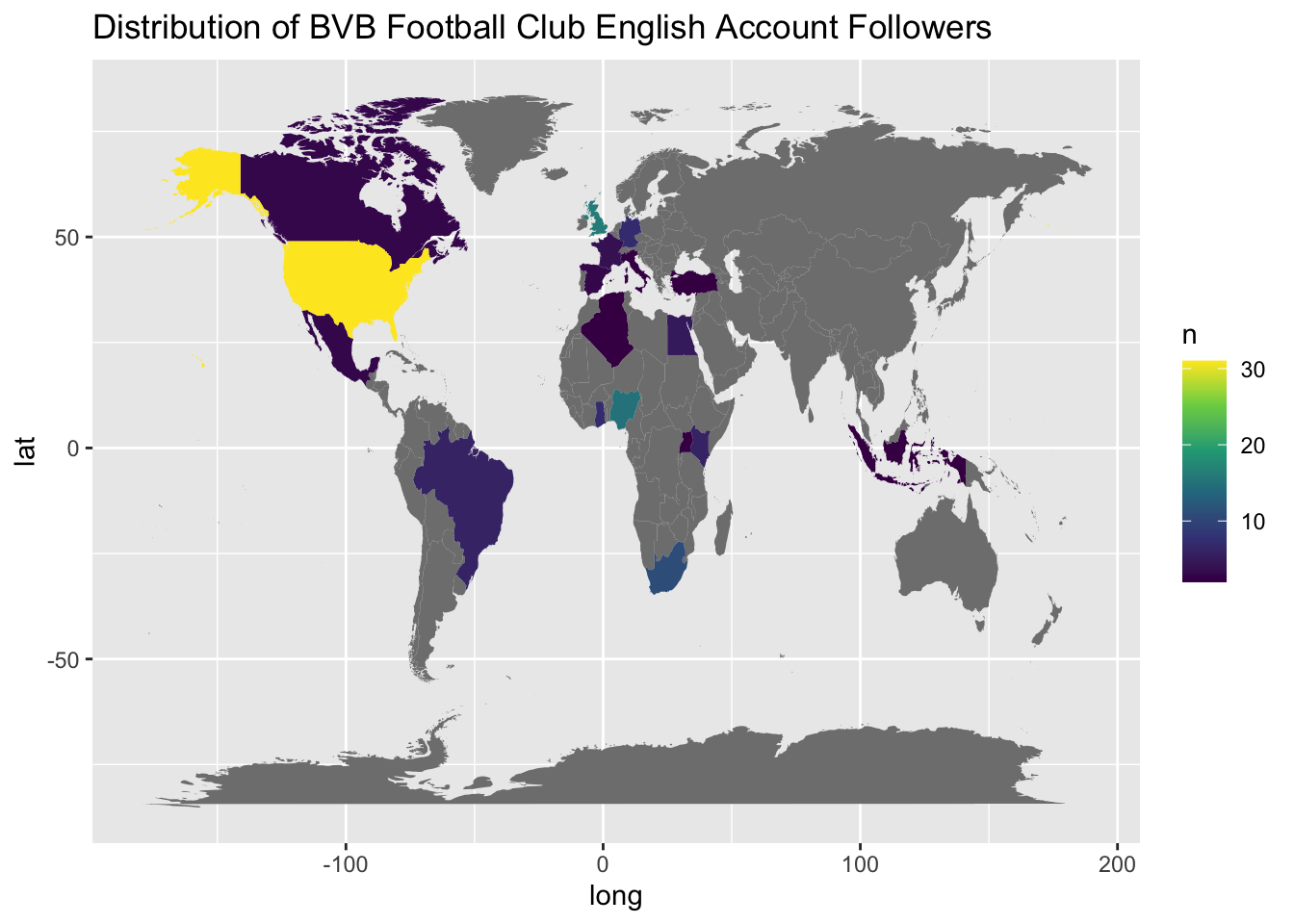
The largest countries of followers in the sample are US, UK and Nigeria. The wider population for BVB followers of the English language account may be significantly different as the first 500 accounts are pulled, which is not a representative sample. Additionally, many followers of BVB’s tweets follow sister accounts in different languages, such as the primary German language Twitter handle.
   followers_agg <- followers_geo %>%
      count (country) %>%
      filter (country != "NOT LISTED", n > 1) %>%
      arrange (-n)

   ggplot (followers_agg, aes (x = reorder(country, n), y = n)) +
      geom_col () +
      coord_flip () +
      theme_minimal() +
      labs (x="", y = "Followers")
Visualize followers on a map
Next we will convert to a map to enable viewing the location of all users along with countries with most users.
   library (maps)

   world <- map_data ("world") %>%
      mutate (region = str_to_upper (region)) %>%
      left_join (followers_agg, by = c("region" = "country"), keep = T)

   world %>%
      ggplot () +
         geom_map (map = world, aes (x = long, y = lat, map_id = region, fill = n)) +
         scale_fill_viridis_c () +
         theme_grey () +
         labs (title = "Distribution of BVB Football Club English Account Followers") +
         ggsave ("bvb_map.png", width = 11)
4. Potential future analyses
We are only scratching the surface of available Twitter data, subsequent data enrichment from complementary packages and subsequent analytics. Second generation followers (followers of followers) could easily be sourced and subtotaled to identify possible impact from a tweet. Or Twitter users that the account itself follows could also be extracted. Another idea is to convert the R code to Shiny to enable interactivity to efficiently change Twitter handles.
5. Conclusion
R offers many powerful tools to source, analyze and visualize Twitter information. The Twitter API (accessed via the rtweet package) enables free sourcing of follower and tweet attributes that can be easily imported into R. The raw data can then be enriched by sourcing geographic attributes from Google’s API via the ggmap package. Tidyverse package such as dplyr, ggplot and GT can then be leveraged to transform and visualize for insight.