Motivation
Spotify is an amazing app to play favorite music, discover new music and rediscover old favorites. In addition, the Spotify API provides free access to a wide array of data on songs, which R users can leverage via Charlie Thompson's spotifyR package. I wanted to learn more about my musical tastes while learning new R skills.
1. Activate Spotify connection
First step is to sign up for a free Spotify API developer ID and secret token.
Next we install the spotifyR library.
Finally, you can either embed the Spotify login information directly in the script or assign to an enivronment variable. The advantage of an environment variable is your private login information will be stored on your computer. That way your R code can be shared without exposure to your login information being stolen. The usethis package simplifies creating and updating environment variables.
   library (spotifyr)

   access_token <- get_spotify_access_token(
      client_id=Sys.getenv("SPOTIFY_CLIENT_ID"),
      client_secret=Sys.getenv("SPOTIFY_CLIENT_SECRET")
      )
2a. Source favorite song statistics
I decided to focus my analysis on liked tracks (called "favorites" in the Spotify API). The get_my_saved_tracks function extracts all liked songs along with basic information such as artist(s), album name and album release year.
Spotify limits the number of tracks per call to 50, much less than my 159 favorites. A clever workaround by Han Chen is to extract multiple tranches of 50 songs the purrr map function.
The output is a bit unwieldy because contains three layers of nested lists. The highest level is the list is the overall structure. The next layer is the 4 data frames of 50 records produced by each iteration of the map function. The most granular layer contains a mixture of data formats from logical to character to integer to lists. Track.album.artists field is in an example of the "list" variable type becuase multiple artists are assigned for some songs.
Simplifying to a manageable one level list format enables greater flexibility. I consolidated the four 50 record lists into one via the reduce function. I converted the multiple artists per track to separate rows which increased the number of records from 159 unique tracks to 170 unique artist/track combinations.
   library (tidyverse)

   favorite_tracks_stats <-
        ceiling(get_my_saved_tracks(include_meta_info = TRUE)[['total']] / 50) %>%
        seq() %>%
        map(function(x) {
          get_my_saved_tracks(
             limit = 50,
             offset = (x - 1) * 50)
            }) %>%
        reduce (rbind) %>%   #combines assorted lists generated by map function into one
        unnest (track.artists)      #simplifies list to multiple rows for tracks with two artists

   glimpse (favorite_tracks_stats)
## Rows: 186
## Columns: 35
## $ added_at <chr> "2020-07-07T01:40:59Z", "2020-07-0…
## $ href <chr> "https://api.spotify.com/v1/artist…
## $ id <chr> "2sil8z5kiy4r76CRTXxBCA", "6eoJpTI…
## $ name <chr> "The Goo Goo Dolls", "Live", "Mani…
## $ type <chr> "artist", "artist", "artist", "art…
## $ uri <chr> "spotify:artist:2sil8z5kiy4r76CRTX…
## $ external_urls.spotify <chr> "https://open.spotify.com/artist/2…
## $ track.available_markets <list> [<"AD", "AE", "AR", "AT", "AU", "…
## $ track.disc_number <int> 1, 1, 1, 1, 1, 1, 1, 1, 1, 1, 1, 1…
## $ track.duration_ms <int> 214400, 231133, 368960, 245733, 21…
## $ track.explicit <lgl> FALSE, FALSE, FALSE, FALSE, FALSE,…
## $ track.href <chr> "https://api.spotify.com/v1/tracks…
## $ track.id <chr> "4umYKCvExzDsGJlqCNyRvZ", "3LpnzPx…
## $ track.is_local <lgl> FALSE, FALSE, FALSE, FALSE, FALSE,…
## $ track.name <chr> "Give a Little Bit", "I Alone", "M…
## $ track.popularity <int> 38, 62, 44, 43, 58, 63, 48, 23, 26…
## $ track.preview_url <chr> "https://p.scdn.co/mp3-preview/17b…
## $ track.track_number <int> 1, 3, 4, 1, 5, 8, 8, 3, 9, 2, 10, …
## $ track.type <chr> "track", "track", "track", "track"…
## $ track.uri <chr> "spotify:track:4umYKCvExzDsGJlqCNy…
## $ track.album.album_type <chr> "album", "album", "album", "compil…
## $ track.album.artists <list> [<data.frame[1 x 6]>, <data.frame…
## $ track.album.available_markets <list> [<"AD", "AE", "AR", "AT", "AU", "…
## $ track.album.href <chr> "https://api.spotify.com/v1/albums…
## $ track.album.id <chr> "0nshkyiazdyELKNJuNldoa", "4ZsG3if…
## $ track.album.images <list> [<data.frame[3 x 3]>, <data.frame…
## $ track.album.name <chr> "Live in Buffalo July 4th, 2004", …
## $ track.album.release_date <chr> "2004-11-23", "1994-01-01", "1992-…
## $ track.album.release_date_precision <chr> "day", "day", "day", "day", "day",…
## $ track.album.total_tracks <int> 20, 14, 40, 21, 11, 11, 10, 18, 18…
## $ track.album.type <chr> "album", "album", "album", "album"…
## $ track.album.uri <chr> "spotify:album:0nshkyiazdyELKNJuNl…
## $ track.album.external_urls.spotify <chr> "https://open.spotify.com/album/0n…
## $ track.external_ids.isrc <chr> "USWB10402743", "USRR29442178", "G…
## $ track.external_urls.spotify <chr> "https://open.spotify.com/track/4u…2b. Source favorite song features
The above statistics are useful but perhaps not as interesting as song features such as energy, tempo and valence. Full definitions are available on Spotify's developer site.
Track features are stored in a separate Spotify API table so requires a separate SpotifyR called get_track_audio_features.
The function requires a list of track IDs. As such we need to extract track IDs from the above data frame that used the get_my_saved_tracks function. We can remove duplicates as song attributes are unique at song level.
  favorite_tracks_ids <- favorite_tracks_stats %>%
         distinct (track.id) %>%
         pull (track.id)

  glimpse(favorite_tracks_ids)
## chr [1:178] "4umYKCvExzDsGJlqCNyRvZ" "3LpnzPxkMI6XS4JCbhNeek" ...We now have our list of track IDs required by the SpotifyR get_track_audio_features function.
Spotify limits the number of songs per extract to 100 so another iterative map function is required. The output is a list of two data frames, each with 100 songs.
      favorite_tracks_features_list <-
         seq (1, nrow(favorite_tracks_stats),100) %>%
         map(function(x) {
             get_track_audio_features (favorite_tracks_ids[x:(x+99)])
               })
A list of data frames is awkward to work with, so we use the reduce function to reduce the complexity by a level. The list of two nested data frames converts into one consolidated data frame.
Additionally, we have 49 blank rows that can be removed. The above map function extracted songs in multiples of 100 so only 51 songs in the second iteration.
      favorite_tracks_features <- favorite_tracks_features_list %>%
         reduce(rbind) %>%
         drop_na()

      glimpse (favorite_tracks_features)
## Rows: 178
## Columns: 18
## $ danceability <dbl> 0.557, 0.396, 0.529, 0.581, 0.360, 0.522, 0.747, 0.9…
## $ energy <dbl> 0.951, 0.817, 0.784, 0.874, 0.257, 0.850, 0.448, 0.8…
## $ key <int> 0, 6, 1, 10, 7, 7, 4, 11, 4, 7, 2, 7, 4, 7, 1, 5, 5,…
## $ loudness <dbl> -3.003, -7.282, -5.288, -5.811, -9.655, -4.769, -15.…
## $ mode <int> 1, 1, 0, 1, 1, 1, 1, 0, 0, 1, 1, 1, 0, 1, 1, 0, 1, 1…
## $ speechiness <dbl> 0.0330, 0.0450, 0.0283, 0.0347, 0.0315, 0.0361, 0.06…
## $ acousticness <dbl> 1.94e-03, 2.28e-03, 6.61e-06, 2.21e-02, 1.59e-02, 1.…
## $ instrumentalness <dbl> 1.72e-04, 4.17e-03, 1.42e-01, 2.38e-06, 5.12e-03, 3.…
## $ liveness <dbl> 0.1570, 0.3720, 0.1350, 0.1130, 0.2260, 0.2950, 0.12…
## $ valence <dbl> 0.5280, 0.0992, 0.2530, 0.9470, 0.1300, 0.7100, 0.94…
## $ tempo <dbl> 93.974, 90.264, 112.461, 143.284, 76.972, 124.216, 1…
## $ type <chr> "audio_features", "audio_features", "audio_features"…
## $ id <chr> "4umYKCvExzDsGJlqCNyRvZ", "3LpnzPxkMI6XS4JCbhNeek", …
## $ uri <chr> "spotify:track:4umYKCvExzDsGJlqCNyRvZ", "spotify:tra…
## $ track_href <chr> "https://api.spotify.com/v1/tracks/4umYKCvExzDsGJlqC…
## $ analysis_url <chr> "https://api.spotify.com/v1/audio-analysis/4umYKCvEx…
## $ duration_ms <int> 214400, 231133, 368960, 245733, 212184, 346280, 2196…
## $ time_signature <int> 4, 4, 4, 4, 4, 4, 4, 4, 4, 4, 4, 4, 4, 4, 4, 4, 4, 4…2c. Combine song features and statistics
Spotify assigns an alphanumeric ID code for each song. The ID is in both the statistics and attributes tables so the two tables can be joined together.
A few other housekeeping items are required before proceeding to the the chart. First, Song duration is clearer in minutes instead of milliseconds. Second, I cleaned song titles by removing "Remaster", "Remastered" as well as parenthetical qualifiers. Third, I converted album release year to number of years past 1970 to better visually discern year differences (bar charts typically start at zero).
   library (lubridate)

   favorite_tracks_combine <- favorite_tracks_features %>%
         right_join(favorite_tracks_stats, by = c("id" = "track.id")) %>%
         rename (artist.name = name) %>%
         mutate (
            duration = duration_ms / 1000 / 60,             #converts milliseconds to minutes
            track.name = str_remove (track.name, c("Remaster", "Remastered")),
            track.name = str_remove (track.name,"[(-].+"),
            track.name = ifelse (str_length (track.name) <= 22, track.name, str_extract(track.name, "^.{22}")),
            release = ifelse (
               track.album.release_date_precision == "year",      #some songs only lists years not dates
               as.integer(track.album.release_date),
               year(as_date(track.album.release_date))
               ),
            release = release - 1970                  #enables bar charts to start at 0
            ) %>%
         select (artist.name, track.name, danceability, energy, valence, tempo, duration, release) %>%
         distinct (track.name, .keep_all = T)

      glimpse (favorite_tracks_combine)
## Rows: 177
## Columns: 8
## $ artist.name <chr> "The Goo Goo Dolls", "Live", "Manic Street Preachers", "…
## $ track.name <chr> "Give a Little Bit", "I Alone", "Motorcycle Emptiness ",…
## $ danceability <dbl> 0.557, 0.396, 0.529, 0.581, 0.360, 0.522, 0.747, 0.958, …
## $ energy <dbl> 0.951, 0.817, 0.784, 0.874, 0.257, 0.850, 0.448, 0.880, …
## $ valence <dbl> 0.5280, 0.0992, 0.2530, 0.9470, 0.1300, 0.7100, 0.9470, …
## $ tempo <dbl> 93.974, 90.264, 112.461, 143.284, 76.972, 124.216, 128.5…
## $ duration <dbl> 3.573333, 3.852217, 6.149333, 4.095550, 3.536400, 5.7713…
## $ release <dbl> 34, 24, 22, 36, 46, 15, 7, 43, 43, 19, 18, 18, 19, 23, 4…3a. Create charts by feature
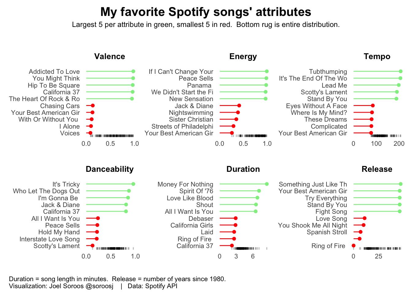
We will create a bar chart for each attribute that represent the top 5 and bottom 5 songs for each attribute. A bottom rug illustrates the full dispersion.
Manually creating 6 charts is inefficient with high inconsistency exposure - not to mention boring. Unfortunately the simpler ggplot facet function generates charts via filtering but cannot sort by variable. Instead I wrote a map function that cycles through each attribute which sorts the metrics and creates the charts.
First step is to create the map function inputs, which are the six variables in the charts.
attributes <- c("valence", "energy", "tempo", "danceability", "duration", "release")Second step is to create the function which calculates the statistics and creates the chart. Each variable iteration of the function sorts songs by attribute, identifies top 5 / bottom 5, creates a bar chart and bottom rug.
   library (glue)

      attributes_plot = function(attribute) {
         attribute = ensym (attribute)
         ggplot (
               data = favorite_tracks_combine %>%
                  arrange (-!!attribute) %>%
                  slice (1:5, (n()-4):n()) %>%
                  mutate (bar_color = ifelse (!!attribute > median (!!attribute), "Lightgreen", "Red")),
               aes (x = reorder (track.name, !!attribute), y = !!attribute),
               size = 1
               ) +
            geom_point (
               aes(color = I(bar_color)),
               shape = 19
               ) +
            geom_segment (
               aes(
                  xend = reorder (track.name, !!attribute), y = 0, yend = !!attribute,
                  color = I(bar_color)
                  )
               ) +
            geom_rug (
               data = favorite_tracks_combine,
               aes (y = !!attribute),
               inherit.aes = F,
               sides = "l",
               alpha = 0.3
               ) +
            scale_y_continuous (n.breaks = 4) +
            coord_flip () +
            theme(
               plot.title = element_text(hjust = 0.5, vjust = 0, size = 10, face = "bold", margin = margin (10,0,10,0)),
               axis.text = element_text (size = 8),
               axis.title = element_blank(),
               axis.ticks = element_blank(),
               panel.grid = element_blank(),
               panel.background = element_blank()
               ) +
          labs (
             title = glue({str_to_title(attribute)})
             )
      }
Finally, we call the map function which sources the above vector input and chart creation function.
The output is a list of charts. These are not yet terribly useful because listed sequentially without titles, subtitles and captions drawing together.
   song_plots <- map(attributes, attributes_plot)
   song_plots
## [[1]]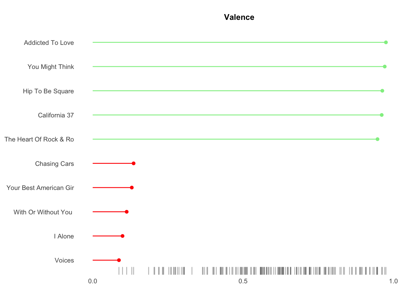
##
## [[2]]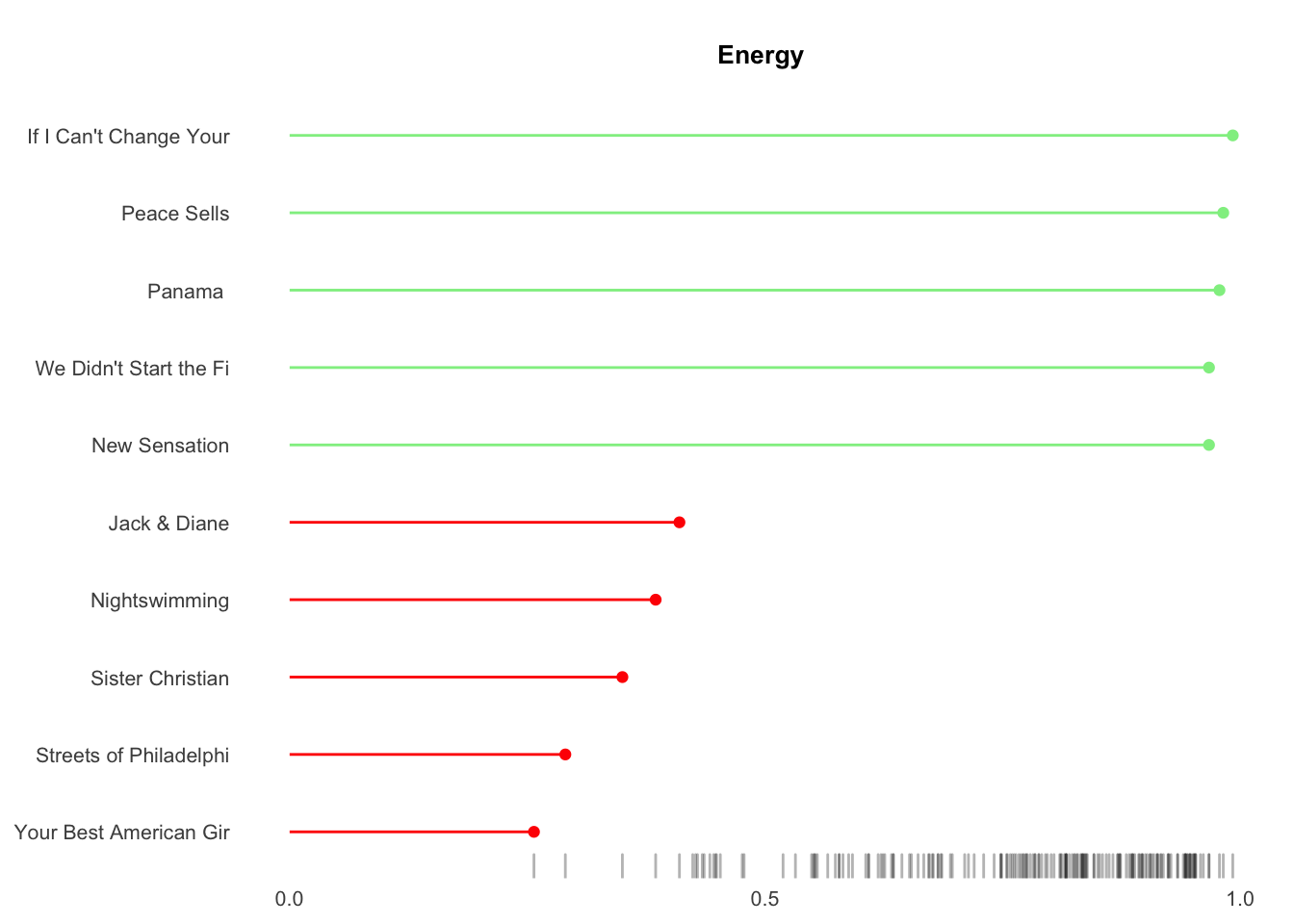
##
## [[3]]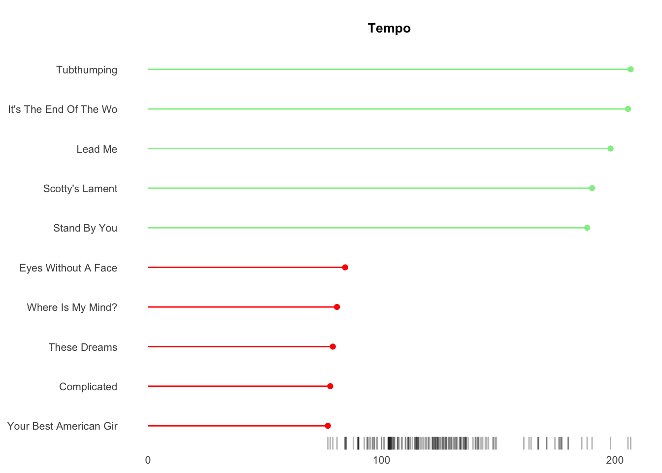
##
## [[4]]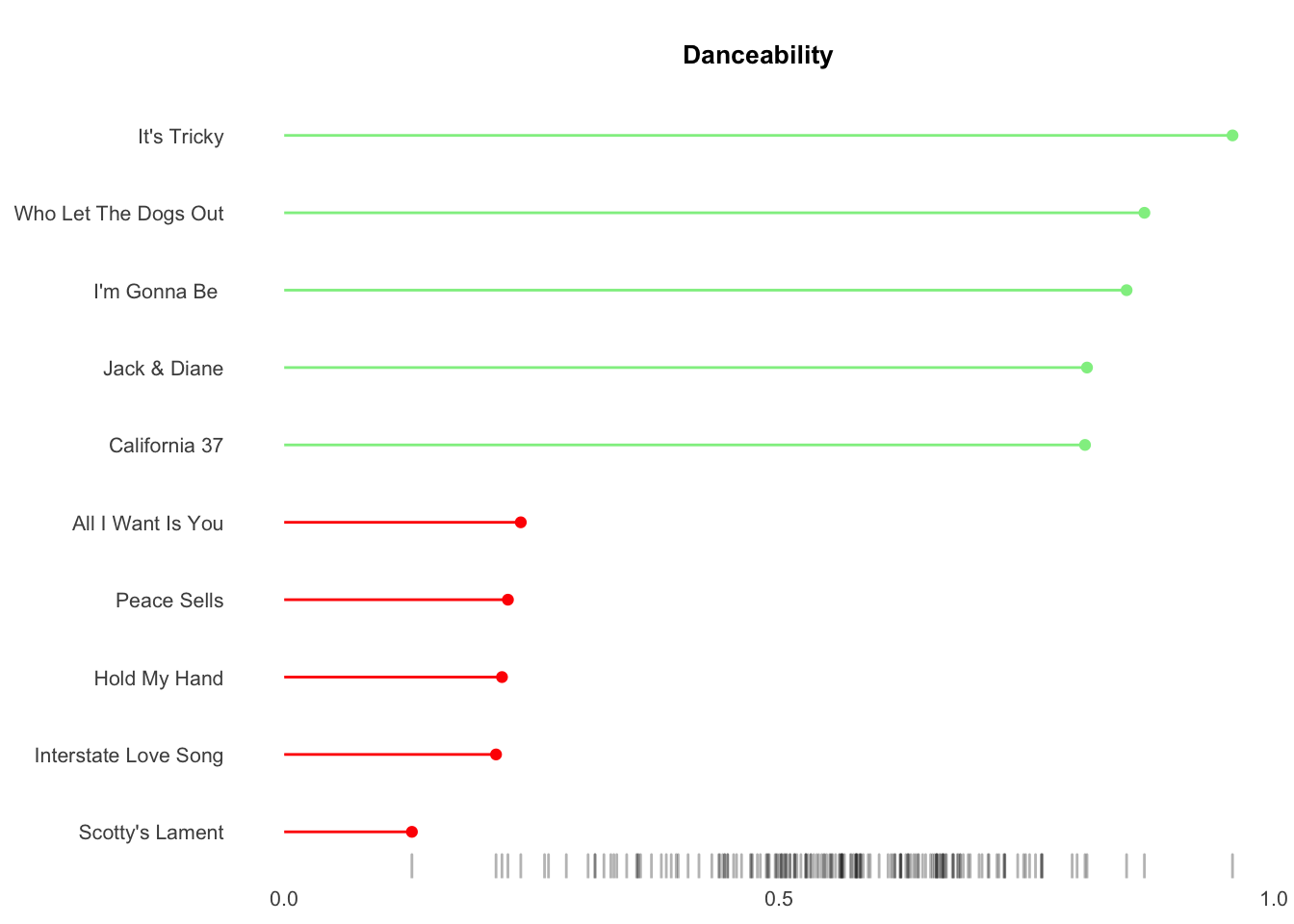
##
## [[5]]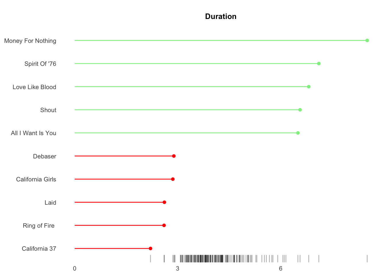
##
## [[6]]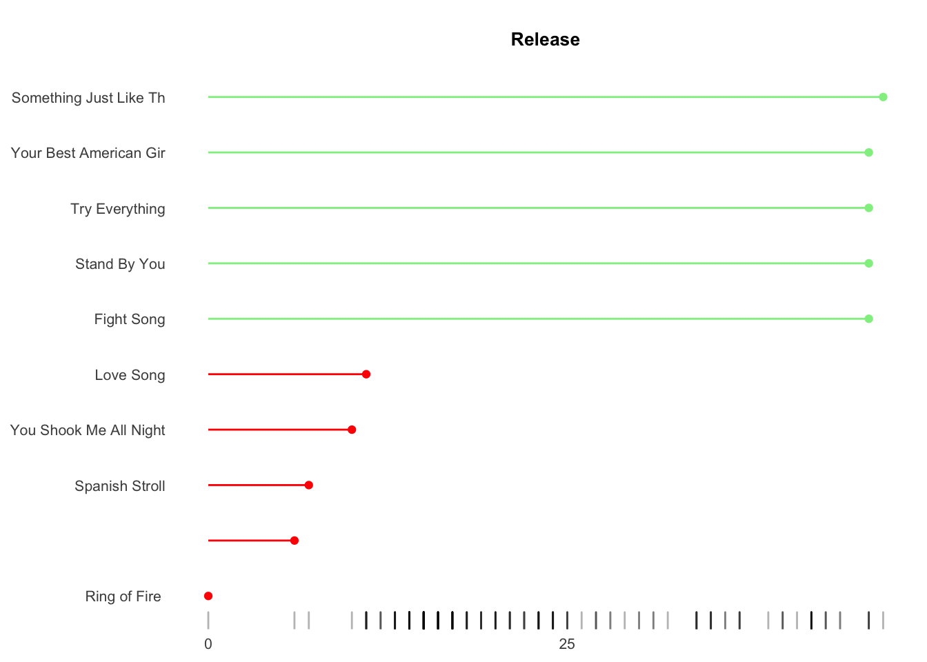
3b. Combine charts, add titles/subtitles/captions
My favorite chart combination package is Thomas Lin Pederson's excellent patchwork package. Charts automatically are aligned vertically and/or horizontally. I have six charts so by default patchwork prints the first three charts on top row then second three on bottom row.
Results show my musical tastes skew toward songs with greater valence (postive emotions), high energy, low tempo, medium danceability, 4-5 minutes of duration and the 1980s.
   library (patchwork)

   #combine charts into grid
      song_plots_combine <-
         song_plots[[1]] + song_plots[[2]] + song_plots[[3]] + song_plots[[4]] + song_plots[[5]] + song_plots[[6]] +
         plot_annotation (
            title =  "My favorite Spotify songs' attributes",
            subtitle = "Largest 5 per attribute in green, smallest 5 in red.  Bottom rug is entire distribution.",
            caption = "Duration = song length in minutes.  Release = number of years since 1980.  \nVisualization: Joel Soroos @soroosj    |   Data: Spotify API",
            theme = theme (
               plot.title = element_text(hjust = 0.5, vjust = 0, size = 15, face = "bold", margin = margin (0,0,5,0)),
               plot.title.position = "plot",
               plot.subtitle = element_text(hjust = 0.5, vjust = 0, size = 9, margin = margin (0,0,15,0)),
               plot.caption = element_text (hjust = 0, size = 8, face = "plain", margin = margin (15,0,0,0)),
               plot.caption.position = "plot"
               )
            )

      ggsave("song_attributes.png", song_plots_combine)
      song_plots_combine